图像分割常用评价指标

转载于https://zhuanlan.zhihu.com/p/117435908,在此致谢

正文

基础知识


如上图,进行医学图像脑肿瘤分割,其中:
T1蓝色部分表示真实脑肿瘤区域(Ground Truth), T0:除T1蓝色外的其它部分为正常脑区域
P1红色部分表示预测的脑肿瘤区域(Prediction), P0:除P1红色的其它部分为预测的正常脑区域

那么评价指标:

  • TP(True Positive):被模型预测为正类的正样本,即蓝色与红色的交集:$T1 \bigcap P1$

    TP(紫色部分)
  • TN(True Negative):被模型预测为负类的负样本,即红色与蓝色以外区域

    TN(紫色部分)
  • FP(False Positive):被模型预测为正类的负样本,即红色中除了蓝色部分

    FP(紫色部分)
  • FN(False Negative):被模型预测为负类的正样本,即蓝色中除了红色部分

    FN(紫色部分)

Dice系数

对于分割过程中的评价标准主要采用Dice相似系数(Dice Similariy Coefficient,DSC),Dice系数是一种集合相似度度量指标,通常用于计算两个样本的相似度,值的范围0-1,分割结果最好时值为1,最差时值为0.

Python代码实现

1
2
3
4
5
6
7
8
9
10
11
12
def dice_coef(output, target):#output为预测结果 target为真实结果
smooth = 1e-5 #防止0除

if torch.is_tensor(output):
output = torch.sigmoid(output).data.cpu().numpy()
if torch.is_tensor(target):
target = target.data.cpu().numpy()

intersection = (output * target).sum()

return (2. * intersection + smooth) / \
(output.sum() + target.sum() + smooth)

IOU:重叠度(Intersection of Union)

IoU分数是对象类别分割问题的标准性能度量。 给定一组图像,IoU测量给出了在该组图像中存在的对象的预测区域和Ground Truth区域之间的相似性,并且由以下等式定义:

其中TP,FP和FN分别表示真阳性,假阳性和假阴性计数。

Python代码实现

1
2
3
4
5
6
7
8
9
10
11
12
def iou_score(output, target):
smooth = 1e-5
if torch.is_tensor(output):
output = torch.sigmoid(output).data.cpu().numpy()
if torch.is_tensor(target):
target = target.data.cpu().numpy()
output_ = output > 0.5
target_ = target > 0.5
intersection = (output_ & target_).sum()
union = (output_ | target_).sum()

return (intersection + smooth) / (union + smooth)

TPR:True Positive Rate(真阳性率)

预测正确的样本占总阳性样本的比例,越大越好.又称为Sensitivity:灵敏度

Python代码实现

1
2
3
4
5
6
7
8
9
10
11
12
def sensitivity(output, target):
smooth = 1e-5

if torch.is_tensor(output):
output = torch.sigmoid(output).data.cpu().numpy()
if torch.is_tensor(target):
target = target.data.cpu().numpy()

intersection = (output * target).sum()

return (intersection + smooth) / \
(target.sum() + smooth)

Precision:精确率

表示预测为阳性的样本中,预测正确的比例,越大越好

Python代码实现

1
2
3
4
5
6
7
8
9
10
11
12
def ppv(output, target):
smooth = 1e-5

if torch.is_tensor(output):
output = torch.sigmoid(output).data.cpu().numpy()
if torch.is_tensor(target):
target = target.data.cpu().numpy()

intersection = (output * target).sum()

return (intersection + smooth) / \
(output.sum() + smooth)

Hausdorff_95 (95% HD)

Dice系数对分割出的内部填充比较敏感,而hausdorff distance 对分割出的边界比较敏感。


下面8张图能够很清晰讲解它的原理:


简言之:
单向:先找最小,再找最大
双向:先找单向,再找最大

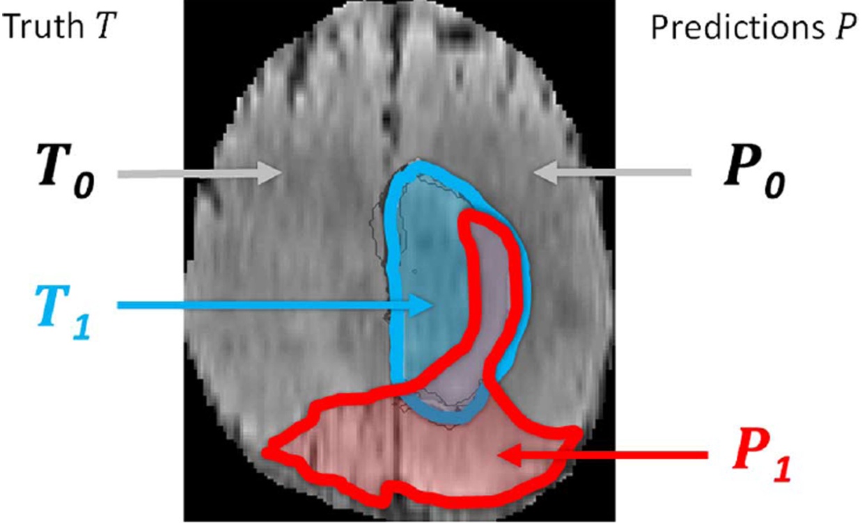
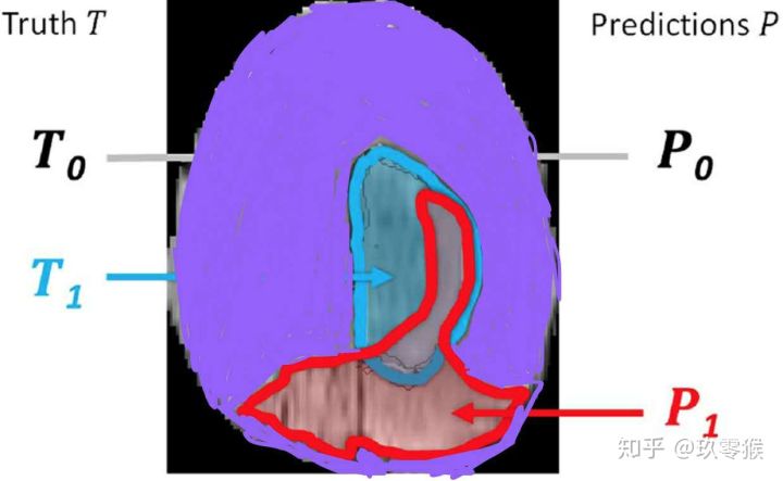
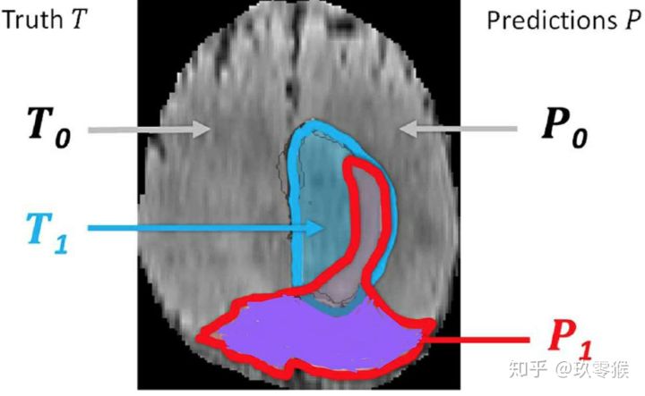
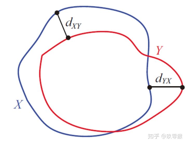
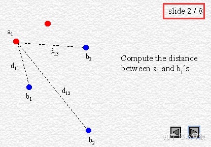
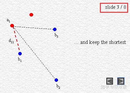
95% HD is similar to maximum HD. However, it is based on the calculation of the 95th percentile of the distances between boundary points in X and Y. The purpose for using this metric is to eliminate the impact of a very small subset of the outliers.

Hausdorff_95就是是最后的值乘以95%,目的是为了消除离群值的一个非常小的子集的影响。
环境安装:

1
2
pip install -i https://pypi.tuna.tsinghua.edu.cn/simple numba
pip install hausdorff

Python代码实现

1
2
3
4
5
6
7
8
9
10
11
12
13
14
15
16
17
18
19
20
21
22
23
import numpy as np
from hausdorff import hausdorff_distance

# two random 2D arrays (second dimension must match)
np.random.seed(0)
X = np.random.random((1000,100))
Y = np.random.random((5000,100))

# Test computation of Hausdorff distance with different base distances
print("Hausdorff distance test: {0}".format( hausdorff_distance(X, Y, distance="manhattan") ))
print("Hausdorff distance test: {0}".format( hausdorff_distance(X, Y, distance="euclidean") ))
print("Hausdorff distance test: {0}".format( hausdorff_distance(X, Y, distance="chebyshev") ))
print("Hausdorff distance test: {0}".format( hausdorff_distance(X, Y, distance="cosine") ))

# For haversine, use 2D lat, lng coordinates
def rand_lat_lng(N):
lats = np.random.uniform(-90, 90, N)
lngs = np.random.uniform(-180, 180, N)
return np.stack([lats, lngs], axis=-1)

X = rand_lat_lng(100)
Y = rand_lat_lng(250)
print("Hausdorff haversine test: {0}".format( hausdorff_distance(X, Y, distance="haversine") ))